Google Nerual Net Quick Draw
Doodling with Deep Learning!
Our Journey with Sketch recognition
![]()
In this blog post, we describe our process understanding, fitting models on, and finding a fun application of the Google Quick, Draw! dataset. Walk with us through this journey to see how we have tackled the challenge of successfully classifying what is "arguably the world's cutest research dataset!"
This project was built by Akhilesh Reddy, Vincent Kuo, Kirti Pande, Tiffany Sung, and Helena Shi. To see the full code used, find our github:
I. Background
In 2016, Google released an online game titled "Quick, Draw!" — an AI experiment that has educated the public on neural networks and built an enormous dataset of over a billion drawings. The game itself is simple. It prompts the player to doodle an image in a certain category, and while the player is drawing, the neural network guesses what the image depicts in a human-to-computer game of Pictionary. You can find more information on the game here or play the game yourself!
Since the release of 50 million drawings in the dataset, the ML community has already begun exploring applications of the data in improving handwriting recognition, training the Sketch RNN model to teach machines to draw, and more. Notably, it has robust potential in OCR (Optical Character Recognition), ASR (Automatic Speech Recognition) & NLP (Natural Language Processing), and reveals lovely insights into how people around the world are different, yet the same.
II. The Data
Our total data size is 73GB with 50 million drawings in 340 label classes. Each drawing comes with specific variables:
- "word" — the class label of that drawing
- "country code" — country of origin of the drawer
- "timestamp" — timestamp of the drawing
- "recognized" — indication of the app's successful prediction
- "drawing" — stroke-base data specific for doodle images; each drawing is made up of multiple strokes in the form of matrices
III. Approach
We began by understanding the structure of arrays that make up a sketch and pre-processing the data. Then, we delve into fitting some simple classifiers and a basic convolutional neural network, or CNN. From there, we tackle CNN architectures such as ResNet and MobileNet. Finally, we shared our results with the world by participating in a Kaggle competition.
Due to the large size of the data and need for a higher capacity GPU, we implemented CNN structures on the Google Cloud Platform, which has a handy free trial with $300 of credits. To find out how we did so, follow links here and here.
IV. Data Preprocessing
The data exists in a format of separate CSV files for drawings of each class label. Therefore, we first shuffled the CSVs, creating 100 new files with data from all classes to ensure the model received a random sample of images as input and remove bias.
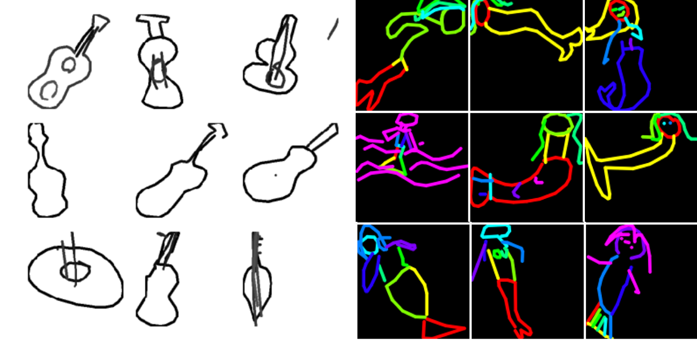
Most people draw doodles in similar ways. For example, if I asked you to draw a sun, you would begin with a single circle, and then dash lines radiating from the center in clockwise order. To capture this information, we used greyscale/color-coded processing to take advantage of the RGB channel while building the CNN so the model could recognize differences between each stroke. We assigned a color to each chronological stroke of a doodle, thus allowing the model to gain information on individual strokes instead of only the whole image.
We also augmented the images by randomly flipping, rotating or blocking parts to introduce noise into the images and increase the capacity of the model to tackle noise. In the course of the game, some players don't finish their doodles or draw in different angles. The augmentation can yield information to the model in those cases.
Both the greyscale/color encoding and image augmentation used OpenCV and ImageGenerator from keras, which loads batches of raw data from csv files and transforms them into images.
V. Building Models
After completing all the data collection and preprocessing steps, it was time to get started on the most interesting part of the project — model building!
Before we dove into CNN, we tried some basic classifiers to compare different machine learning algorithms and familiarize ourselves with the data. We pulled numpy files of the data from Google Cloud Storage. This data has already been preprocessed and rendered into a 28x28 grayscale bitmap in numpy .npy format. Since the entire dataset included over 345 categories, we eventually went with a small subset that only contains the following 5 classes: airplane, alarm clock, ambulance, angel and animal migration.
Random Forest
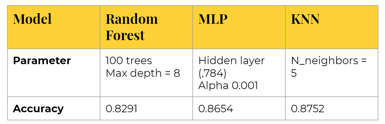
We first began with a Random Forest classifier. We utilized GridSearchCV to cross-validate the model and optimize parameters. We found that accuracy tends to plateau after 100 trees, so we used n_estimators = 100 as our final model, returning an accuracy of 0.8291.
KNN
Secondly, we tried the k-Nearest Neighbor (kNN) classifier, arguably the simplest and easiest model to understand. Its algorithm classifies unknown data points by finding the most common class among the k-closest examples. We cross validated the n_neighbors and found that the best model given is k = 5, which returns 0.8752 accuracy.
Multi-Layer Perceptron (MLP)
Lastly, we tried the Multi-Layer Perceptron (MLP) from scikit-learn. We cross validated over different hidden layer sizes and learning rates, deciding on a hidden layer size of (784,) and learning rate alpha = 0.001, which gave accuracy of 0.8654.
Convolutional Neural Network
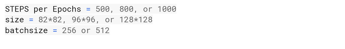
We then moved on to a simple CNN model to set a lower threshold for model performance and understand the nuances and execution time of the model. In this model, we used the drawing information in the data to create an image of the desired size using OpenCV. Here we tried a bunch of different parameters as shown:
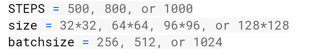
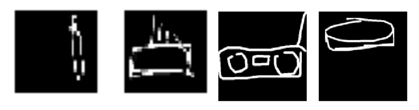
Here is some intuition behind our parameters settings. Firstly, a larger batch size would help in addressing the noise due to mislabeled training data. The size parameter denotes the image size/resolution and has significant impact on accuracy. For example, a comparison of 32x32 and 128x128 shows us that a size of 32x32 is too pixelated to achieve an accurate model.
The first model used two convolutional layers, each with depth of 128. Such an increase in image size, however, required either a larger receptive field conv layer or an additional conv layer. Accordingly, we included one more layer when training with larger image size. Below is the custom CNN model that we created with number of convolutional layers, dense layers, dropout and size as the parameters while building the model.
As we were still deciding on the best model to proceed further with the analysis, we used limited data at the initial step to lessen execution time.
Selecting an Optimizer
A key step before proceeding with training is deciding which optimizer to use. After referring to the literature and taking advice from experts on various Kaggle forums, we decided to compare the performance of the Adam optimizer and the SGD optimizer on our data. After multiple iterations, we chose the Adam optimizer because we observed that it showed slightly better results and converged faster than SGD.
After running the model on 25000 images per class for about 3 hrs, we obtained a MAP@3 score of 0.76 on Kaggle's Public Leaderboard — not a bad result for merely 25000 images per class! To put this into perspective, the average class in the dataset contains 150000 images. However, when we increased the model complexity, the accuracy slightly degraded, which led us to our next step: ResNet.
SE-ResNet-34, SE-ResNet-50:
When increasing the depth of the model, it is likely to face issues like vanishing gradient and degradation; comparatively, deeper models perform worse than simpler ones. A Residual Network, or ResNet is a neural network architecture that solves the problem of vanishing gradients and degradation issue in the simplest way possible by using deep residual learning.
In simple words, during back propagation, when the signal is sent backwards, the gradient always must pass through f(x) (where f(x) is our convolution, matrix multiplication, or batch normalization, etc), which can cause trouble due to the non-linearities which are involved.
The "+ x" at the end is the shortcut. It allows the gradient to pass backwards directly. By stacking these layers, the gradient could theoretically "skip" over all the intermediate layers and reach the bottom without being diminished.

You can refer to the original paper to further understand the comparisons between a 34 layer plain network and and a 34 layer residual network.
In this step of the process, we trained SE-ResNet-34 and 50 as a step further from simple CNN. The term SE refers to Squeeze and Excitation Net; with it, an additional block gives weights to different channels. The SE blocks were proven to provide additional accuracy by giving the weights yet merely increased less than 10% of total parameters. More information on Squeeze & Excitation Nets can be found here.
While training of SE-ResNet-50, we tried different parameters as the following for 50 to 60 epochs.
Finally, out of all the combinations, the batch size of 512 and image size of 128x128 gave the best improvement to the score, boosting it to 0.9093. It is important to note that changing the batch size and image size is based on the GPU that we were using and that these were the maximum possible parameters on Tesla k80 for our data.
MobileNet
After multiple iterations with SE-ResNet and with the competition deadline quickly approaching, we decided to explore MobileNet, which gave comparable accuracy yet executed much more quickly.
MobileNet was introduced by Google to enable the delivery of the latest technologies such as object, logo, and text recognition for customers anytime, anywhere, irrespective of Internet connection. MobileNets are based on a streamlined architecture that uses depth-wise separable convolutions to build lightweight deep neural networks.
To put this into perspective, a standard convolution does the application of filters across all input channels and the combination of these values in a single step. In comparison, a depthwise separable convolution performs two different steps:
- Depthwise convolution applies a single filter to each input channel
- Pointwise convolution, a simple 1×1 convolution, is then used to create a linear combination of the output of the depthwise layer
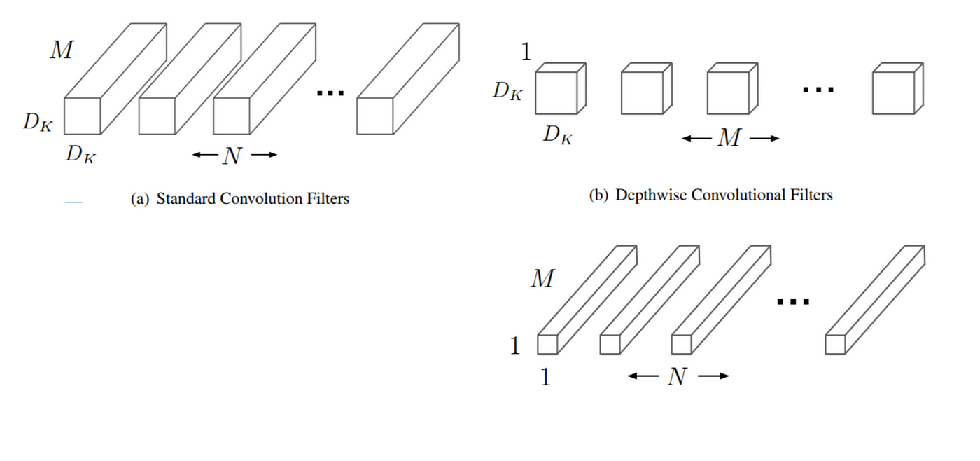
This factorization drastically reduces computation and model size as it breaks the interaction between the number of output channels and the size of the kernel. According to the original paper on MobileNet, MobileNet showed a reduction in computation costs by at least 9 times. For further details, you can refer to the original paper on MobileNet.
For simplicity's sake, we used the simple, 2-line, standard module of MobileNet in keras.
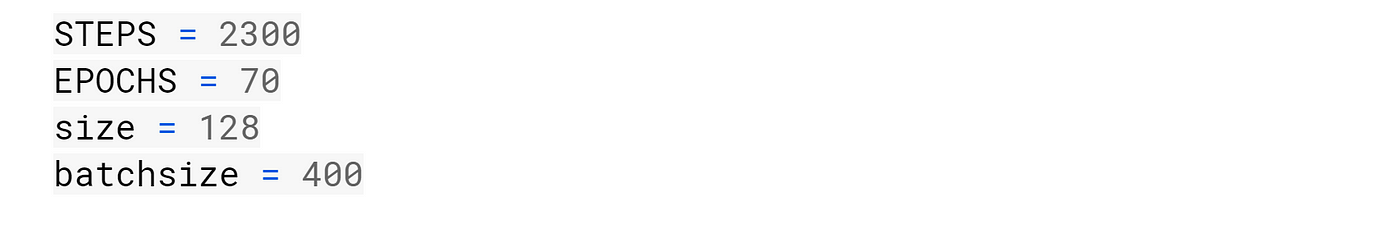
Before training the mode, we ensured that we used all 50 MM images to train the model and included the order of stroke information through a greyscale gradient for each stroke. After multiple iterations, we came upon the following parameters as optimal parameters.
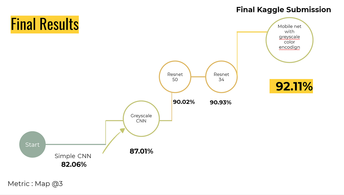
VI. Results
We began training the model on 50MM drawings and 340 classes on a Tesla P100 GPU provided by Google Cloud platform. After training for 20 hours and spending $50 of GCP credits, we finally reached a score of 0.9211 using MobileNet on the Kaggle leaderboard, which helped us secure a rank of 268 among the 1316 teams that participated in the competition!
Here you can see an overall summary of our models' parameters and results:
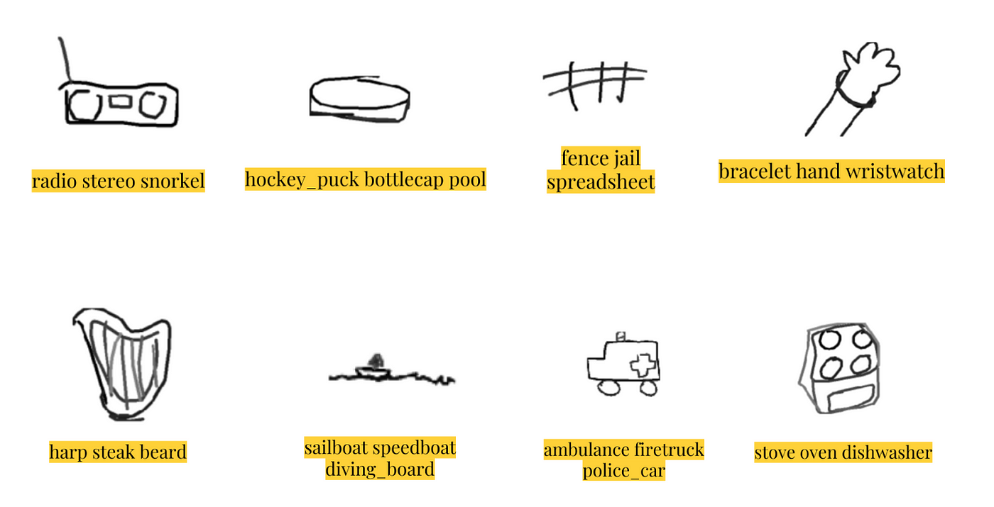
Following are some examples of our predictions!
A Fun Bonus!
If you've stuck it through and read to this point, extra points for you! As a fun treat, we decided to also spice things up a little and created an application that could capture doodles via webcam! The app used our model to carry out predictions in real time. OpenCV functions were utilized to capture the video from the webcam and extract the images drawn.
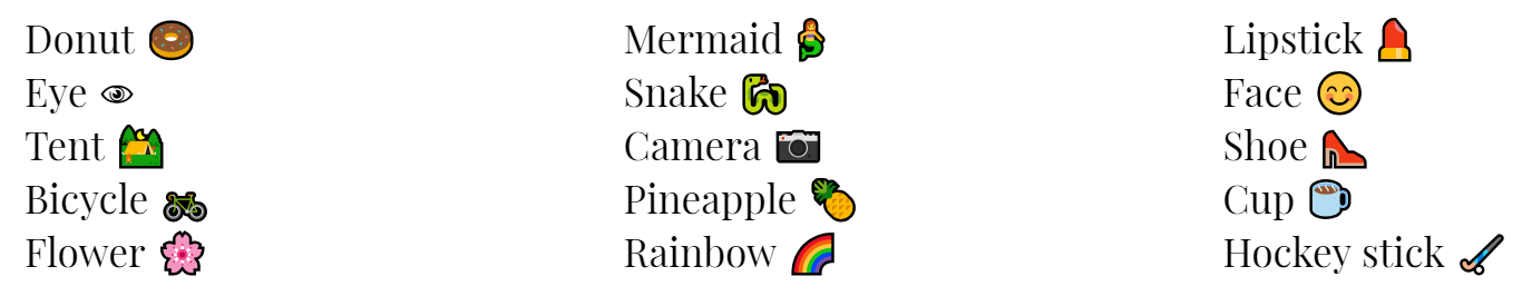
We used the first Simple CNN model as our back-end since it was the lightest model we had run. The model is trained on the 15 classes (listed below) and achieves an 87% accuracy to detecting the doodle drawn.
VII. Conclusion
As a conclusion, we'll summarize the steps taken in this winding journey:
- Wracked our brains to understand the unique structure of doodle data and figured out how to connect with Google Cloud Platform to run the models
- Performed data cleaning & preprocessing through shuffling csvs and augmenting images with stroke information and more
- Ran reduced dataset of five classes on three simple classifiers on our local system
- Implemented Deep learning models from a simple CNN to ResNets and MobileNets
- Submitted results to the competition, gave ourselves a big pat on the back, and celebrated the end of the project by creating an app!
Following are some lessons learned while training a deep learning network:
- Get one basic implementation of the algorithm and test it on a smaller dataset first to save execution time
- Explore all the available GPU options and alternate between them based on the computational intensity that is required for the task
- Reduce learning rate with increases in epochs. We have a built in function called ReduceLRonplateau to perform this operation. This impacts the learning of the model during the plateau
Overall, this project was incredibly rewarding! As graduate students, we seized the opportunity to both (hopefully!) impress our professor and participate in prestigious competition. We were able to challenge ourselves by tackling image classification for the first time and came out with more than satisfactory results.
References
None of this work could have been done on our own. Check out the following references to get access to all the great resources we used:
https://cloud.google.com/blog/products/gcp/drawings-in-the-cloud-introducing-the-quick-draw-dataset
https://ai.googleblog.com/2017/04/teaching-machines-to-draw.html
https://www.kaggle.com/c/quickdraw-doodle-recognition
https://www.blog.google/technology/ai/quick-draw-one-billion-drawings-around-world/
https://www.kaggle.com/gaborfodor/shuffle-csvs
https://www.kaggle.com/remidi/simple-strokes-to-rgb-kernel
https://www.kaggle.com/titericz/black-white-cnn-lb-0-782
https://www.google.com/url?q=https://stats.stackexchange.com/questions/148139/rules-for-selecting-convolutional-neural-network-hyperparameters&sa=D&ust=1544740608219000&usg=AFQjCNGwJl5GpZwWpKmpFclt6qiNwwQnHA
http://ruder.io/optimizing-gradient-descent/index.html#adam
http://cs231n.stanford.edu/reports/2016/pdfs/264_Report.pdf
https://chatbotslife.com/resnets-highwaynets-and-densenets-oh-my-9bb15918ee32
https://www.kaggle.com/jpmiller/image-based-cnn
https://console.cloud.google.com/storage/browser/quickdraw_dataset/full/numpy_bitmap//
https://github.com/akshaybahadur21/QuickDraw
https://chatbotslife.com/resnets-highwaynets-and-densenets-oh-my-9bb15918ee32
Source: https://towardsdatascience.com/doodling-with-deep-learning-1b0e11b858aa